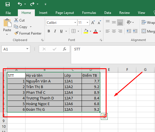
Bước 1: Bôi đen vùng dữ liệu bạn cần tô màu.
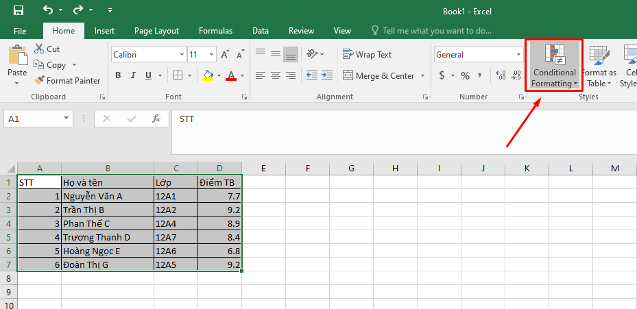
Bước 2: Chọn Conditional Formatting để bắt đầu định dạng có điều kiện.
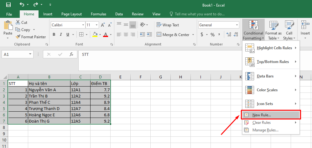
Bước 3: Chọn New Rule… tạo định dạng mới theo nhu cầu của bạn.
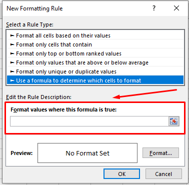
Bước 4: Chọn Use a formula to determine which cells to format trong phần Select a rule type.
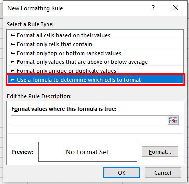
Bước 5: Tại ô Format values where this formula is true, bạn tiếp tục nhập công thức muốn dùng để định dạng tô màu cho ô.
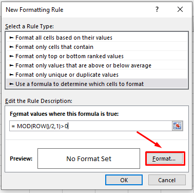
Bước 6: Ví dụ để tô màu ô xen kẽ, ta dùng công thức =MOD(ROW()/2,1)>0, sau đó chọn Format.
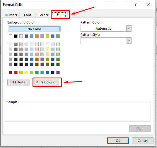
Bước 7: Chọn mục Fill để lựa chọn màu cho ô.
Lưu ý: Bạn có thể lựa chọn màu sắc tùy thích bằng cách chọn More colours…
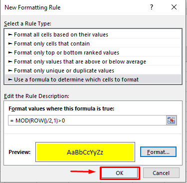
Bước 8: Nhấn OK và hoàn thành.
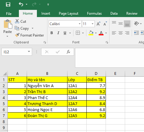
Ta nhận được kết quả sau khi thực hiện tô màu ô theo điều kiện.
Thanh Trà